
Perspective on Risk - Oct. 25, 2022 (Economics)
r*; R*; r**, g>r; Financial Repression; Productivity
I’m not an economist; strangely, throughout my career, many folks have assumed I was. But I do play one on Substack sometimes. I thought it might be useful to review some current observations on things like r*, R*, r** and g.
This is long; I’ve tried to explain things as simply as I can given my understanding. 99% of you will hate this and probably should ignore it, and the other 1% will tell me how I am wrong! I certainly might have some things wrong and I hope the economists in the audience will correct me if I’m off base. I’ll also warm you that the post sort of peters off at the end - didn’t end with a conclusion I was happy with.
r*
What is r* again?
Economists consider r* the ‘natural’ rate of interest, and generally define it as
the the inflation-adjusted, short-term interest rate that is consistent with full use of economic resources and steady inflation near the Fed’s target level.
The recent interest traces back to a paper by Laubach and Williams Measuring the Natural Rate of Interest Redux.1 At the time it was written, John Williams was the President of the San Francisco Fed, and he’s now the President of the New York Fed. So it matters because all of the central bankers will talk about it from time to time.
Economists use these estimates to help inform the setting of interest rates, and the financial markets measure where the level of market rates are relative to their estimates of r* to determine if they think monetary policy is loose or tight.
The NY Fed maintained a web-page that shows some estimates of r*, but suspended it due to Covid (and has not yet turned it back on - boo). r* had made a low of 0.21% in 2014 (according to the LW formulation of the model), rose slowly back to >1%, and then collapsed again with Covid.
The IMF2 recently included an estimate (based on a slightly different model, the Holston, Laubach, Williams model3 using a Kalman filter4).
 / Twitter")
The IMF states:
it seems possible that the natural rate may have increased slightly, loosening the stance of policy further (Figure 1.24), although there is still a great deal of uncertainty about the natural rate at medium- and long-term horizons.
This, of course, matters because if central banks are to use tight monetary conditions to slow demand, the fact that the ‘natural rate’ may have risen means they will need to continue tightening rates longer than otherwise. The problem is that there is such a range of error to the estimates that it will be difficult to truly know if the rate is ‘tight’ absent observing the effect on the economy (which will introduce a lag to their response function).
Fidelity’s Jurrien Timmer has published his estimates of r* and the resulting real rate of interest. I find this graph interesting because it purports to show the cyclicality of monetary policy.


His terminal real rate of ~3.25% is generally consistent with a subsequent recession.
R* (not to be confused with r*)
The Bank of England published an interesting staff working paper Decomposing the drivers of Global R*5 . In a paper we will subsequently discuss, Andrew Bailey states R* is the trend component of r*, which is labeled as R*.6 They create a structural model that treats the world as a single large (closed) economy, populated by overlapping generations of finitely-lived households. Their model includes five observable drivers of R∗:
productivity growth,
population growth,
longevity,
the relative
price of capital and government debt.

What are the conclusions?
Our simulations show that Global R∗ rises from 1.25% in the mid-1950s to around 2.75% in the mid-1970s. Thereafter, Global R∗ declines steadily, reaching −0.25% at the end of our sample in 2015. In the early part of our sample, higher productivity growth and population growth (the ‘baby boom’) raise Global R∗. The subsequent decline is predominantly driven by falling productivity growth and increased longevity. The relative price of capital has only a modest effect on the equilibrium real interest rate and, at a global level, movements in trend government debt are not sufficient to have a material impact on R∗.
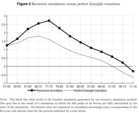
The results are then summarized in this excellent chart:

The estimated decline in Global R∗ from its peak has been primarily driven by changes in longevity and productivity growth. Increased longevity, due to rising survival probabilities in particular for over-65s, raised the stocks of wealth that households wish to hold to fund their retirements. Higher desired wealth holdings have in turn reduced Global R∗. Slower trend productivity growth has also reduced Global R∗, since lower expected returns on investment have reduced the demand for capital.
Higher population growth in the early part of our sample (the ‘baby boom’) pushes up slightly on Global R∗, with the effects particularly noticeable in the 1990s and 2000s. Thereafter the effect wanes but not sufficiently to push down on R∗ in our model. In line with other studies (e.g., Sajedi and Thwaites, 2016), the relative price of capital has only a modest effect on the equilibrium real interest rate. Finally, at a global level, according to the calibration of our model, trend movements in government debt are not sufficient to have a material impact on R∗.
I personally find it hugely interesting that the level of government debt has had little to no effect on the trend component of the ‘natural’ rate.
Next, the Bank of England’s Andrew Bailey gave a speech The economic landscape: structural change, global R * and the missing-investment puzzle where he discusses a recent paper Structural change, global R* and the missing-investment puzzle7 that he authored with BoE colleagues. The paper extends the earlier paper by focusing on an apparent empirical observation that excess profitability has not led to a commensurate increase in investment.
He begins with framing:
For an open economy like the United Kingdom, the trend real rate is pinned down by global forces; as capital is free to move around the world, interest rates would depend on the balance of savings and investment in other countries as well as the United Kingdom. Global R* thus acts as a long-term anchor for the UK’s domestic equilibrium real interest rate. Understanding the relative importance of the different secular factors that drive Global R*, therefore, sheds light on the forces that may ultimately shape the evolution of domestic real interest rates.
Global estimates of R* have been falling in recent years, but over the longer term look bounded between 0 and ~3%.

He then discusses work done by the Bank on the structural drivers of R* and shows the sensitivities that they found:

I will skip some of the details (but you really should read the speech or paper). Bailey then lists his observations and conclusions:
what this model, and the data behind it, are telling us is that we should not expect that ageing, and the retirement of baby boomers, will lead to significant upward pressure on Global R* over coming years or decades.
Standard neoclassical theory, … implies a strong co-movement between the safe real rate and rate of return on capital. This suggests that we would expect a fall in Global R* to be associated with a fall in the return on capital. But while risk-free rates have been falling globally in recent decades, measures of the rate of return on productive capital across high-income economies have not.
… this wedge, between the return on firms’ investment and the cost of financing it, is a measure of firm profitability. As such, it is a key determinant of investment. Accordingly, we might expect to have seen an increase in investment activity alongside the recent increases in the wedge. But, while the wedge has increased, across the same group of countries, … investment has steadily declined, or, at best, remained stable
What accounts for this? It’s not particularly clear.
In contrast with the existing literature studying the United States, the results find little role for changes in competition. For the United Kingdom, intangible investment plays the most important role.
r**
OK, now that you have r* and R* down, let’s add another * and talk about r**. Economists at the NY Fed have written a paper The Financial (In)Stability Real Interest Rate, R**8
They define r** as
a financial stability real interest rate using a macroeconomic banking model with an occasionally binding financing constraint. … The financial stability interest rate, r**, is the threshold interest rate that triggers the constraint being binding.
The goal is to define r** such that
if the real rate in the economy is at or above r**, the tightness of financial conditions may generate financial instability
The construct of the model is frankly beyond my understanding, but the observations and implications are not.
In response to a fall in real interest rates, the share of safe assets plummets, … giving rise to a positive correlation between x and the real rate. Lower safe asset ratio, in turn, gives rise to an increase in financial frictions faced by the bank, contributing financial vulnerabilities to build up.
Stability breeds instability.
low interest rates are associated with a lower ratio of safe-to-risky assets in the banking sector. This buildup of risky lending moves the economy closer to the financial stress region.
Or as Ed Price puts it in a nice writeup9 of the paper in layman’s terms.
Financial stability ≠ macroeconomic stability. R-star ≠ r-star-star.
During periods of financial stress, r** < r*. That is, the necessary ‘natural rate’ for financial stability is below that estimated for macro-economic stability.
By construction, r** is below r during periods of financial stress, and above it otherwise, although the uncertainty is often large enough that that the intervals include r. Broadly speaking, it appears that during the first part of the Great Moderation period, in the mid to late 80s and the 90s, r** is significantly above r except for short-lived episodes of stress such as the LTCM crisis. In the 2000s and right after the Great Recession the gap between r** and r is close to zero, meaning that the constraints is close to being binding, even in periods that are not classified as financial stress episodes. In the mid to late 2010s r** is generally well above r, except again for a couple of very short-lived periods of stress, until the Covid pandemic hits the economy in March 2020. We also note that in most financial stress episode r** is rarely if ever significantly below r for extended periods of time, with the Great Recession being the only exception, when monetary policy was constrained by the zero lower bound.
The paper has this key conclusion:
in reality, crises are eventually triggered by several other factors including a deteriorating TFP levels so that the relationship between low real interest rates today and future crisis is far from mechanical and is difficult to use in trying to predict the timing of crises.
g > r
Once upon a time, a French economist, Thomas Piketti, wrote a rather lengthy book, Capital in the 21st Century that many people bought and promptly left on their coffee tables unread. I didn’t bother to buy it, but have read summaries.10 According to Wikipedia:
The book's central thesis is that inequality is not an accident but rather a feature of capitalism that can be reversed only through state intervention.
Economists from the NY Fed summarized his arguments in a 2015 blog post11 as:
The main argument in Capital for why wealth inequality is set to rise comes from a simple relation: r > g. This formula states that the net rate of return to capital (r) exceeds the growth rate of output (g). This is not a new concept for economists. The formula r > g is a standard property of efficient capital markets in most modern macroeconomic models.
Great, blah blah, blah. I get it. Brian why are you wasting my time with this?
Well, it’s because @jasonfurman has been pointing that we may be at or approaching an inflection point. We have been in a regime where g>r for quite a while after the 2008 global financial crisis.
At times when g>r governments *should* debt-finance expenditures because the debt diminishes as a burden over time. The Federal Reserve projects the long term growth rate of US GDP to be in the 1.6 - 2.2% range.12


As Furman points out:
Fidelity’s Jurrien Timmer has a nice way of showing whether Fed policy is inflating or deflating financial assets. Looking at the below chart, TIPS break-even spread (horizontal) on the nominal yield (vertical). The blue line is a simple regression of the two, using the 2008-2019 period as in-sample. Being above/below the regression line projects whether the Fed is tight/loose.

Here is an alternative way of displaying the information. If you believe this analysis, the move fast, break things approach taken by the Fed is resulting in the tightest financial conditions since the GFC. You will note from the chart below that the two past tightenings have lasted for about two years.

Productivity
OK, so it took a long time to get here, I hope you are still with me. In all of the above sections, productivity has been a key issue/input. It helps explain the decrease in R*, it affects the Piketty r>g argument, and it affects the degree to which the policy rate is set tight or loose.
So what’s going on with productivity?
There has been some noise about some recent data showing a drop in productivity. Here is one such example (not to pick on @MacroAlf, he’s a smart guy)


So let’s step back. The Bureau of Labor Statistics published statistics on total factor productivity (TFP), and decomposes the results into labor and capital components. Their latest report13 was published in August and covers through 2021. While there has been some recent noise associated with the Covid shutdown, it appears that TFP has only increased by about 5% since 2010.

This has been commented on by others, including Steven Rattner.


The SF Fed has a useful page summarizing recent reports, and it has a useful download of all of the needed statistics.
I took a look at their labor productivity numbers. There of course is a lot of noise from the GFC and Covid. I fitted a 4th order polynomial (red line; for no particular reason ) to see if there is a trend, and it looks like there is a 2% decrease in labor productivity from the 2008 GFC onward. I’d probably disregard the recent downturn unless more evidence emerges.

Now, at least theoretically, real interest rates are a determinant of private investment. The desired capital stock inversely related to the cost of capital. A decrease in the real interest rate lowers the opportunity cost of capital and, therefore, raises the desired capital stock and investment spending.
So let’s look at the recent history of the capital input to labor productivity. A rising cost of capital, represented by positive real rates, ought to affect this going forward. Here it is below (again with a 4th order polynomial fitted in red).

It does appear as if there was a pretty sizeable decrease in the growth contribution following Y2K, and perhaps a slight decrease following the 2008 GFC.
I didn’t do any statistical tests, but there doesn’t appear to be a correlation between the peaks/troughs of Jurrien Timmer’s financial repression graph (proxy for real rate tightness) and the peaks/troughs of capital input. The higher level of capital input does extend back to around 1995.
I did scan the literature and did not find much real information. Economists from the Chicago Fed published Understanding global trends in long-run real interest rates in 2017. Their paper tends to run the causality from the capital contribution to labor productivity to the level of real interest rates. At best, they find some support for long-term real rates measured over a decade affecting capital investment, sometimes.
Perhaps a more interesting paper is The circular relationship between productivity growth and real interest rates14. They posit that there is a circular relationship between total factor productivity (TFP) growth and real interest rates that contributes to secular stagnation, and persists until there is a technology shock.
Anyway, I hate to end on an inconclusive note.
It strikes me that we are in a bit of a conundrum: we need policies (fiscal and monetary) that increase supply while constraining demand, all while increasing productivity.
Laubach, Williams, Measuring the Natural Rate of Interest Redux
Holston, Laubach, Williams, Measuring the Natural Rate of Interest: International Trends and Determinants
A Kalman filter is a way of de-noising estimates.
Cesa-Bianchi, Harrison and Sajedi, “Decomposing the drivers of Global R*”, Bank of England staff working paper 990
In the August 2018 Inflation Report, the MPC set out its framework for thinking about the equilibrium interest rate, which is also described in further detail in a background paper co-authored with Bank staff that will be published alongside this speech. That framework decomposes the equilibrium real interest rate, sometimes called r*, into the sum of two components. The first component, called the ‘trend real rate’ or upper-case R* for short, is driven by long-term structural factors. The second component of (lower-case) r* reflects the effects of cyclical shocks to both aggregate demand and supply and so can vary substantially over the short to medium term.
Bailey, Cesa-Bianchi, Garofalo, Harrison, McLaren, Piton, and Sajedi, “Structural Change, Global R* and the Missing-Investment Puzzle,” Bank of England
Akinci, Benigno, Del Negro and Queralto, The Financial (In)Stability Real Interest Rate, R**
Price, Financial instability wants its money back, Financial Times
It’s not that I have an aversion to long books; I have actually read Infinate Jest, which clocks in at 1,077 pages
Pinkovskiy, A Discussion of Thomas Piketty’s Capital in the Twenty-First Century: By How Much Is r Greater than g?, Liberty Street Economics blog
Summary of Economic Projections, Federal Reserve
TOTAL FACTOR PRODUCTIVITY – 2021, Bureau of Labor Statistics
Bergeaud, Cette, Lecat, “The circular relationship between productivity growth and real interest rates” VoxEU